DETAILS

The following is a brief description of the data visualization presented here. The data are calculated using the coarse-grained approach to MD simulations as implemented in the MARTINI model. The simulation setup we use is documented in detail by Heligi et al. and Corradi et al. It has also been used by Marino et al.

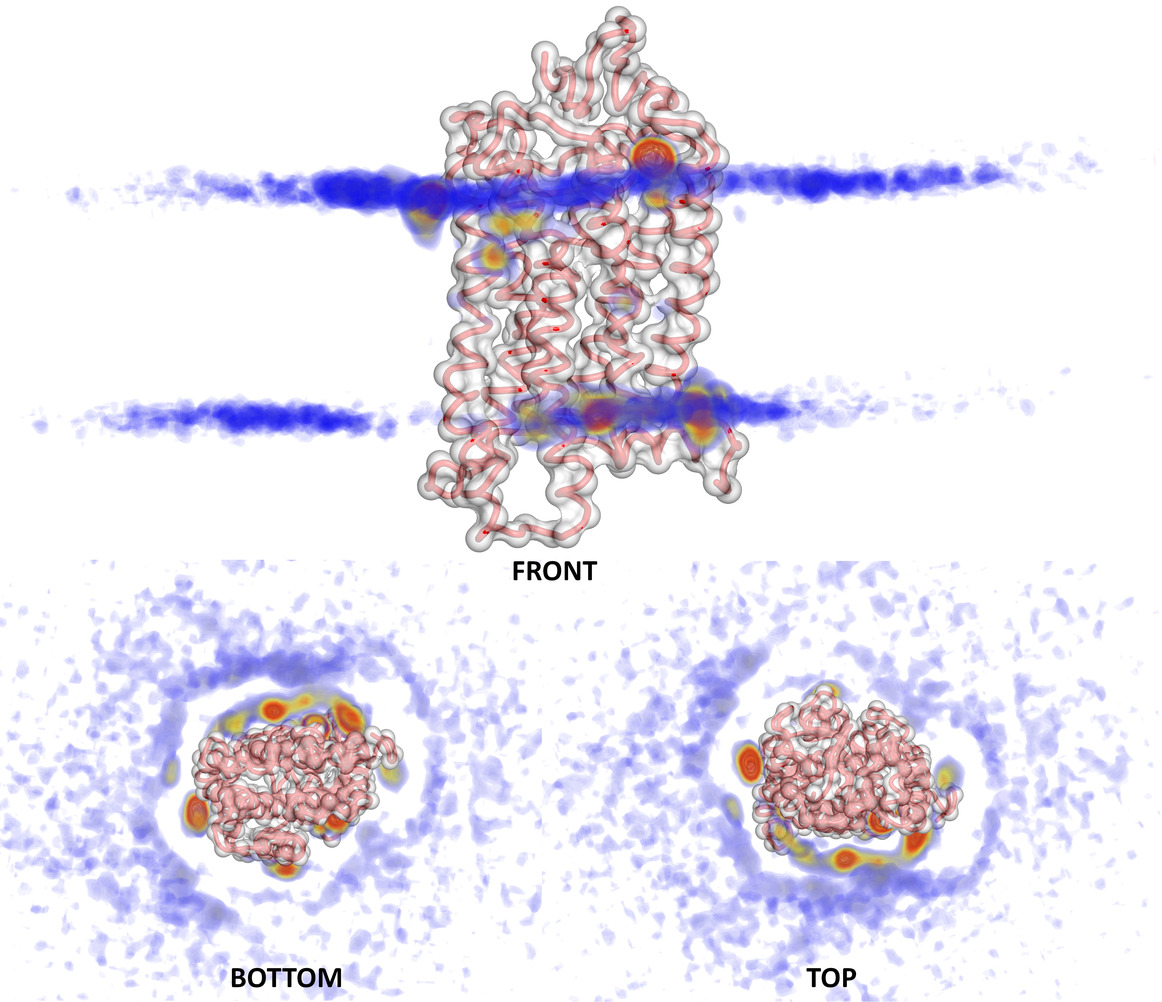
Here, we mainly show 3D density data for cholesterol and phosphatidylinositol phosphates (PIPs) lipids' interactions with G Protein - Coupled Receptors. For the 3D density calculations we only consider lipids within a 6 nm radius around the proteins. In the video below cholesterol molecules (represented by enlarged ROH beads in red) that fit this criterion for one of the proteins are displayed. Blue and red surfaces indicate the position of GM lipids and other cholesterol molecules, repsectively. A higher resolution video is available here.

The data presented here are calculated using the VolMap utility implemented in VMD. A simple code snippet to calculate dx densities starting from a GROMACS trajectory and only selecting the CP beads of PIP lipids is only a few lines of code:

  import numpy as np
  import mdtraj as md
  from gridData import Grid

  traj = md.load('trajectory.xtc', top='coordinates.gro')
  PIPs_ndx = traj.topology.select("(resname =~ 'POP[1-3]') and (name CP)")
  PIPs = traj.xyz[:, PIPs_ndx, :]

  H, e = np.histogramdd(PIPs.reshape(PIPs.shape[0] * PIPs.shape[1], 3), bins=(80, 80, 40))

  g = Grid(H, edges=e)
  g.export('density.dx')

Averaging over the four copies we have in our systems is also quite straightforward (considering our system design, it only makes sense to average in the lateral dimension):

We use the ngl viewer to visualize the data in several representations. Cholesterol and PIP lipids are shown in pink and dark magenta, respectively. The default surface representation is smooth, but other otions are also available. Using the control key and the mouse scroll wheel you can change the isolevels of the surfaces (either each lipid individually, or both of them simultaneously). The slice representation of the density is usefull because it eliminates the need to scroll and fine-tune the lipid surfaces. You can "slice" the 3D density of lipids in the x, y, z direction for each lipid, resulting in the familiar 2D surfaces. When viewing the slice representation, make sure to toggle off the density of that particular lipid, so that it does not interfere with the visualization.

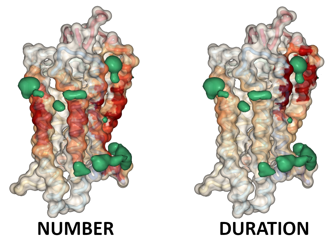
The average number of contacts of GPCRs with cholesterol and PIP lipids as well as the average duration of those contacts is shown as a surface coloring of the protein where an increase in the intensity of the color red corresponds to increased number and duration of contacts, respectively. The labels of each protein residue are also shown with the relative size of the label corresponding to their number and duration of contacts, respectively. To view labels make sure to first show either the DURATION or NUMBER maps first.

Visualization programs like PyMOL support a more advanced coloring scheme of 3D densities as shown in the example below for Rhodopsin. You can differentiate regions of higher density (yellow and red here) by a different color compared to regions of lower density (blue in the example below).

PyMOL visualization of Rhodopsin-Cholesterol density isolevels.

Lastly, we display both the average number of contacts for each residue with cholesterol and PIP lipids as well as the average duration of the longest contact formed between them. In the figure below you can see how accounting for the longevity of contacts allows us to clearly identify binding sites. Currently we only show these calculations for cholesterol.

Neither method is superior. Plotting contact durations will give fewer interaction sites, and much more pronounced maximum vs minimum levels. It accentuates the most localized interaction spots. The average number of contacts are more difficult to interpret, but they give a better picture of how involved residues are in making contacts with cholesterol.

Not necessarily! They should give an overall agreement but the 3D density is calculated for only the ROH bead of cholesterol, whereas a "contact" is considered for the whole cholesterol molecule. It is, however, quite easy to infer the overall alignment of cholesterol in the binding sites from just the ROH bead density.

The issue lies on the low concentration of PIP lipids. Any given putative binding site for PIP lipids, contains usually 1, 2 or maybe 3 lipids at any given time. Since, in our calculations of the PIP lipid 3D density we only consider the CP beads, that leads to there being only a few data points per frame and as such the result will be less well-defined.

The slice representation is just a different way of visualizing the lipid density. Because lipids are free to move in the simulations in all directions, they will form small undulations on the bilary. The slice representations will capture this motion.

We have used the same protocol to calculate the densities for all GPCRs, and as such, the localization of cholesterol/PIP lipids should be directly comparable. It is, however, not easy to get a measure of the binding strength, especially if we want to compare binding sites in-between different GPCRs. A significantly higher isosurface value for cholesterol, for instance, for one GPCR indicates a "stronger" binding compared to a lower isosurface value for another GPCR. However, this is not guaranteed, and it is unclear what "significantly higher" in this context means.
We also plot the number and duration of contacts formed with cholesterol for each residue, and these results are even more difficult to compare between different GPCRs in terms of binding strength. In fact, we try to avoid this comparison. That is why, for instance, the slider to display the labes, where the size of the label corresponds to either the number or duration of contacts depending on the map being visualized, is reset everytime a new representation is displayed or GPCR is loaded.

VISUALIZATION DETAILS

REFERENCES